2 Activity 2
2.1 The shape of data
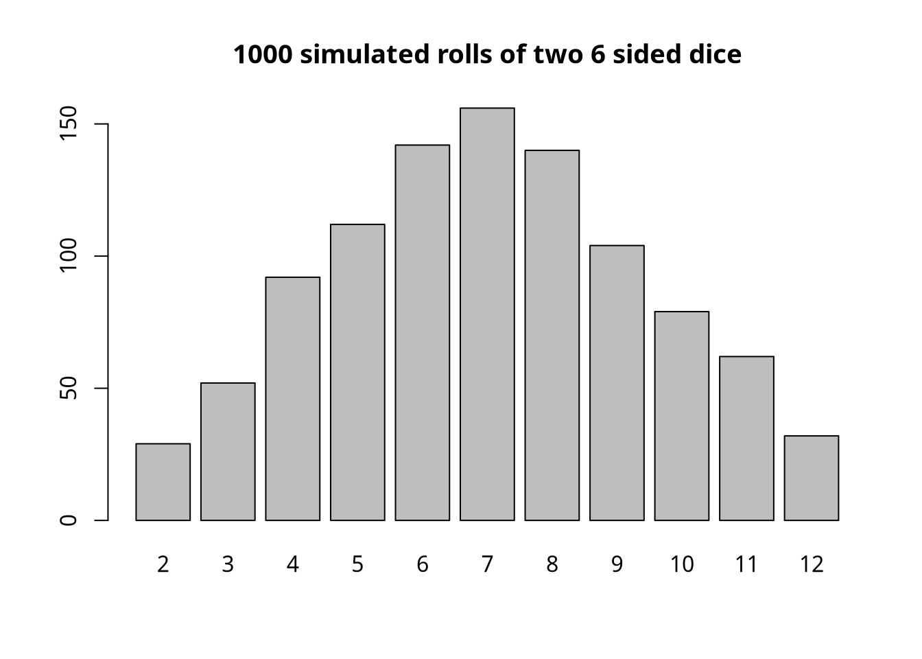
Recall from Activity 1 we made a bar graph of the results we get from rolling two 6 sided dice. As an example, simulating \(1000\) rolls, I generated the following bar graph.
Exercise 2.1
- Take one or two 12-sided dice. Roll them and create a tally of the number of 1s, 2s, 3s, etc. you get. Do this until you have recorded 50 values. So if you have two dice that’s 25 rolls, recording two numbers each roll.
Report your tallies on your lab submission. You do not need to report the bar graph.
- Does your bar graph have a similar shape to the graph for two 6 sided dice?
- One way to smooth out a bar graph is by grouping neighboring values into the same bin (i.e. a histogram). Take your tallies from part (1) and make a table of the number of 1s and 2s, 3s and 4s, 5s and 6s, etc.
- Make a bar plot (histogram) of this combined tally. No need to sketch this but would you describe the shape of this data to be reasonably uniform? (Note: it might not be with only 50 rolls!)
2.1.1 Histograms
The faithful dataset contains data on the length of eruption times and waiting times in between eruptions for the Old Faithful geyser in Yellowstone National Park.
We’ll start by asking R to show us what’s in the variable:
Observe that there are two columns: eruptions (time of each eruption in mins) and waiting (time to next eruption in mins). Let’s extract these variables and use a histogram to help us picture the data.
Exercise 2.2
- Notice that the data doesn’t have just one hill but two hills to it. What is the name for this shape of data?
- Use the
summaryfunction and report the median and mean of each column.
Is the amount of data near the respective means/medians high or low?
Go back to the histograms and change
histtoboxplotfor both eruption time and waiting time. Do these box plots do a good job of conveying the shape of the data?
2.1.2 Scatter Plots
One question you could ask when seeing the Faithful histograms is whether longer waiting times lead to longer eruption times. In order to visualize that question, we’re going to need to plot both variables at the same time. The tool for this is the scatter plot which puts a point at each \((x, y)\) coordinate where \(x\) is waiting time and \(y\) is an eruption time.
Exercise 2.3
- Per the scatter plot, are points which have a lower waiting time (further to the left) associated with a higher or lower eruption time (up/down)?
- If the waiting time to the latest eruption is 80 minutes, about how long does the trend line predict the eruption time will be? (roughly)
Note
We will discuss scatter plots in more detail later in the course.
2.2 Box plots
The nottem data set records the monthly average air temperatures at Nottingham Castle from 1920 to 1939. Which for this exercise we will call just “the monthly temperature.”
Next, we will use box and whisker plots to compare the median temperatures per month. If we just called boxplot(nottem) right now, it would do a single boxplot of the entire data set.
(This is where LLMs can be helpful in telling us how what functions can help separate the data by month.)
Exercise 2.4
- In which month is the highest monthly temperature observed?
- Reading the plot, what are the top 5 months in order sorted by the median of their monthly temperatures? Note: the median is the thick line in the middle of the box.
- It’s a bit hard to compare January and December at the moment, change the last line to read
boxplot(temperatures[,c("Jan", "Dec")])and then state- which of these two months has the higher median monthly temperature and
- which has the lowest overall monthly temperature.
Now let’s look at the numbers.
- Between January and December, which has the greater mean monthly temperature?
- For this particular data, would you say the means are generally close to or far from the medians?